
Next Generation Reservoir Computing - Correctness
What is next generation reservoir computing?
This is a new-ish type of algorithm. It's very good at predicting the next state of a dynamical system.
What is a dynamical system, you say? It's a system where the state at time T can be entirely derived from its state at time T-1. Imagine a cannon ball. We know the equations driving the position of the ball, so if we know the position at T, we can calculate the position at T+1. It's a dynamical system, where the state is the position of the ball in the air.
Now, this example is fairly straightforward, but some systems are way more complex, and the next generation reservoir computing (NGRC) algorithm is very good at learning the underlying set of rules of the system (its equations). We don't even need to know what they are ourselves, only that the system is dynamical!
You can find the research paper here: Next Generation Reservoir Computing, by Daniel J. Gauthier, Erik Bollt, Aaron Griffith and Wendson A.S. Barbosa.
This article is the first in a series that will aim at exploring what can be done with it.
Lorenz Attractors
I am sure some implementation exists in different languages. However, as I said before, I like using Go. I have recently generated my own linear algebra library, and on top of it a new go framework called goblas-ai. The whole thing started with me wanting to explore NGRC in Go!
The LLM did a good job at generating the ngrc algorithm, but the idea here is to really understand how it works, so we will dive more into it.
One way to do that is to try to assess the quality of the AI's implementation. My understanding is that the state of the art to do so is to try to predict the state of a Lorenz attractor.
What is[...] Yes I know, I know. Here is what I understood: you know when one boils some water to cook pasta? The stove heats up the water at the bottom of the pot. The water then moves up, which brings colder water to the bottom, which heats up, etc, etc. You can learn more in this wikipedia article: Convection (Heat Transfer).
Anyway, the same thing happens to all fluids all the time. That's where wind comes from, if you ever wondered. The atmosphere is made of layers. When two adjacent layers don't have the same temperature, the air will move around, which moves the next layer, etc, etc, until it reaches the ground. In the pot, the water at the bottom also creates a separate layer from the cooler water above.
The Lorenz system focuses on three properties of those fluid layers:
- how fast the fluid is circulating (the water moving up and down)
- the temperature difference between the fluid moving up and the fluid moving down
- how much the movement of the fluid has also mixed the temperatures (sometimes, big "blobs" of heat will rise up fast and find themselves surrounded by cold fluid).
It gives us three equations, telling us how those properties evolve in time. Of course, it is only a simplified version. The whole thing was actually designed to make a point: it explains why weather is so hard to predict long term.
In order to do that, the equations contain three parameters introduced to get some variability. Let's go over them:
- How fast does the fluid's speed change when the temperature changes
- How hard we are heating the fluid
- How fast the temperature of the overall layer goes back to equilibrium
The equations are:
<how fast the fluid is moving at T+1> = <how fast the speed changes with temperature> . (<temp difference between fluid up and down> - <how fast the fluid is moving at T>)
<temp difference between fluid up and down at T+1> = <how fast the fluid is moving> . (<how hard we are heating the fluid> - <how mixed up temperatures>) - <temp difference between fluid up and down at T>
<how mixed up temperatures are at T+1> = <how fast the fluid is moving> . <temp difference between fluid up and down> - <how fast temperatures are returning to equilibrium> . <how mixed up temperatures are at T>
Now, depending on the parameters' values, we can observe different patterns regarding the evolution of the layer's state. The most impactful is how hard we are heating the fluid.
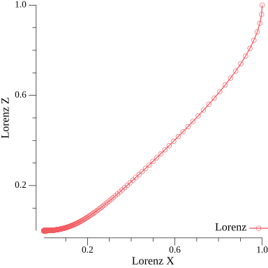
For values less than 1, there is no convection happening, only conduction (just like in a bar of metal, for example). Eventually, the whole state converges to zero. Zero movement, zero temperature, zero everything. Here is a plot showing this happening:
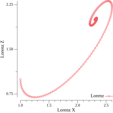
If it is greater than 1, we see two fixed points appear. Those are steady convections. They will converge towards a stable state and get closer and closer to it. We call such a state an "attractor". Here are two examples, using exactly the same parameters but different initial coordinates.
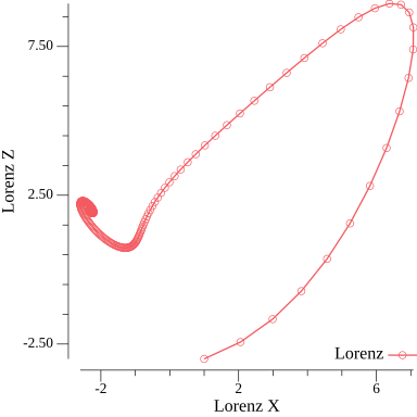
But wait! If we increase the value up to around 24.74 (I don't know why this value in particular), something cool happens: the system becomes chaotic! Concretely, it looks like the system is converging towards an attractor, just like before, but then will unpredictably jump to a second attractor, and again, and again. This creates a famous "butterfly" shape.
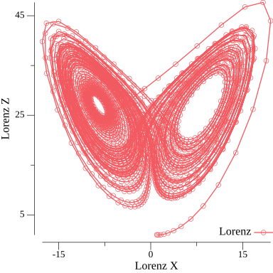
Note that in the plots 1, 2 and 4, we started at the exact same coordinate, but the system behaves very differently depending on the parameter values (especially how hard we heat the fluid).
Correctness Verification
Alright, so the idea is to try to predict the chaotic state of a Lorenz attractor. Apparently it's very hard (because of its chaotic nature), and NGRCs are surprisingly good at it. Let's try it!
First, we need to specify what "good" mean. As we saw, this is a chaotic system, so it is quite unreasonable to expect a perfect long term prediction. So what counts as reasonable?
There is something called a Lyapunov time. It defines how long a system can remain predictable. For example, Pluto's orbit is 200 million years, but the rotation of the 4th moon of Saturn (Hyperion) is only 36 days! From what I read, good forecasters will be able to keep predicting a chaotic system for 5 to 8 Lyapunov times. So, our correctness verification has two steps: calculate how long is our lorenz system's Lyapunov time, and compare it to how long our forecaster remain close enough to the real value.
Calculating the Lyapunov time of the system
The idea is to run two systems side by side. One is considered the original, the second one is a "twin". The twin is starting at a location very, very slightly different from the original one. Then we create a distance accumulator, and we check the degree by which the two systems diverge. By construction, the accumulator should converge towards a certain value (the "rate" at which the systems diverge). Here is a go function to calculate it:
// sigma, rho, beta are the Lorenz parameters
// dt is the step the system increases by
// steps in the number of steps we will run the system for
// transient is the number of steps we will ignore in our calculations to let the attractor settle
func largestLyapunov(sigma, rho, beta, dt float64, steps, transient int) float64 {

	// this is the reference Lorenz system
	lor1 := LorenzSystem{
		State: LorenzState{X: 2, Y: 2, Z: 2},
		Sigma: sigma,
		Rho:   rho,
		Beta:  beta,
	}

	// we create a twin of the first system, starting at a tiny, slightly different location.
	// since it is a chaotic system, the more steps we take the more they will diverge
	d0 := 1e-9
	lor2 := LorenzSystem{
		State: LorenzState{X: 2, Y: 2 + d0, Z: 2},
		Sigma: sigma,
		Rho:   rho,
		Beta:  beta,
	}

	// now we run both systems at the same time and we accumulate the distance between them.
	// as we accumulate the distance, we "pull" the twin system back towards the original one to prevent the distance from being too big
	normalizedDist := 0.0
	for step := range steps {
		lor1.Update(dt)
		lor2.Update(dt)

		// distance between the 2 systems
		euclidianX := (lor2.State.X - lor1.State.X) * (lor2.State.X - lor1.State.X)
		euclidianY := (lor2.State.Y - lor1.State.Y) * (lor2.State.Y - lor1.State.Y)
		euclidianZ := (lor2.State.Z - lor1.State.Z) * (lor2.State.Z - lor1.State.Z)
		euclidianDist := math.Sqrt(euclidianX + euclidianY + euclidianZ)

		// scaling back the twin system
		scale := d0 / euclidianDist
		lor2.State.X = lor1.State.X + (lor2.State.X-lor1.State.X)*scale
		lor2.State.Y = lor1.State.Y + (lor2.State.Y-lor1.State.Y)*scale
		lor2.State.Z = lor1.State.Z + (lor2.State.Z-lor1.State.Z)*scale

		// distance accumulator
		if step >= transient {
			normalizedDist += math.Log(euclidianDist / d0)
		}

	}

	lyapunov := normalizedDist / (float64(steps-transient) * dt)
	return lyapunov
}
Once we have this value, the actual Lyapunov time is 1 over the value returned by this function. To make sure that the implementation is correct, we can run it using different dt and number of steps for the same Lorenz parameters and make sure they always seem to converge properly.
In my case, the value is around 1.240.
go run ./lorenz
Pick what you want to do:
	1. Export the lorenz attractor's values
	2. Train the model from ./lorenz-training-data.csv
	3. Run the lorenz attractor and the model side by side and export to ./lorenz-predictions.csv
	4. Compute the mean squared error from ./lorenz-predictions.csv

4
Lyapunov time is: 1.239960 for dt=0.010000, steps=20000 transient=1000
Assessing the predictions quality
The idea now is to compute the Normalized Root Mean Squared Error (NRMSE) for each time step, and check when it goes over 0.4. We count the number of steps it took to get over this threshold, and make sure that we are staying on track for more than 5-8 Lyapunov times!
Running this, I found that the specific implementation of reservoir computing stayed accurate for 8.95 Lyapunov times! 5+ is considered very good, so we can say that our model is good, and ready to be used on real data!
================ MODEL QUALITY REPORT ================
samples: 2000   sampling dt: 0.0250   horizon: 50.00 time units
Lyapunov time: 1.240
valid for 444 steps = 11.100 time units = 8.95 Lyapunov times (NRMSE crossed 0.4)
I hope this was interesting and helpful. If you are interested in the small program I used to do all those steps, let me know and I can share a link.